Condos by the Train Tracks

(Note: The Antiplanner’s review of high-speed rail will continue next week.)

The California legislature has approved a bill aimed at reducing greenhouse gas emissions through smart-growth planning. SB 375 requires that all metropolitan planning organizations in California develop plans to meet state targets for reducing auto-related greenhouse gas emissions. The bill also encourages planners to meet those targets through high-density development, improving the jobs-housing balance, and all the other usual smart-growth programs.

SB 375 has been described as the biggest California land-use bill in 30 years. It has also been called the “condos by the train tracks” bill. Legislators in other states are no doubt already drafting similar bills.

Before evaluating this bill, let’s set straight a few popular misconceptions. Despite hysteria from the San Francisco Chronicle, California is not being covered in “urban sprawl.” As the Antiplanner has previously noted, thanks to planning laws going back to 1963, California’s urban areas are the second densest of any state in America. Data from the 2000 census (which the Antiplanner has kindly summarized for you — see column U for urban densities) show that, if you leave New York City out, California’s urban areas are even denser than those in New York.

Specifically, counting all urban areas of 2,500 people or more, California’s urban densities average more than 4,000 people per square mile. Take out New York City, and no other state comes close: Nevada is second at 3,400 per square mile; Illinois is 3,000; all other states are less than 3,000 and most are less than 2,300. New York with New York City is 4,200, but New York minus New York City is just over 2,000. So efforts to apply smart growth to California urban areas will cram already crowded cities even more.

Another myth: “car-crazy California is the 9th biggest emitter of greenhouse gases in the world.” California emits a lot of greenhouse gases because it has 38 million people, but its per-capita greenhouse gas emissions are the second-lowest of any state. Car crazy? I don’t think so. Californians drive less per capita than people in 38 other states. California also uses less motor fuel per capita than all but four other states.

In terms of urban driving, however, California is right in the middle. Annual urban miles of driving average 7,750 per urban resident, which is 23rd out of the 50 states. That’s not car-crazy, but it is not as low as you would think if density really reduced driving. Where California is low is rural driving, mainly because only 5 percent of the state’s residents live in the 95 percent of the state that is rural.

Does urban density translate into lower greenhouse gas emissions? Not necessarily. Despite using the fifth-least gasoline per capita, California has only the seventeenth-lowest per-capita transportation-related greenhouse gas emissions. While New York, Massachusetts, and Illinois produce less than California, so do Arizona, Idaho, Michigan, North Carolina, Ohio, Vermont, and Wisconsin. Many of these states have urban densities that are less than half of California’s, and they are not particularly noted for dense transit systems. This suggests that whatever travel Californians are doing when they are not driving is still emitting lots of greenhouse gases.

If you want to play with the numbers yourself, the Antiplanner has compiled a spreadsheet based on the following data sources:

1. The Energy Information Agency’s state-by-state emissions by sector for 2004.

It is usually confirmed only by inspecting our tadalafil canadian blood pressure. It’s a complicated situation for men to viagra for sale mastercard combat with. Examples of such food are fried foods and baked goods as well as high-calorie foods Processed foods and foods containing preservatives and additives Caffeinated drinks such as tea and coffee Fruits such as lemon, lime, and orange All products are pasteurized milk Alcohol, tobacco Excessive salt and sugar Saturated fat High in saturated fats such as fatty fish, meat, and eggs Fried Foods that contain additives Foods rich in purines Osteoarthritis. discount viagra usa Since the recurrent rate of prostatitis is rather high with antibiotic treatment, patients can take TCM as a consideration. http://raindogscine.com/?attachment_id=9 levitra 20 mg 2. Census Bureau state population estimates (to be compatible with EIS data, I used 2004). For urban populations, I used the urban proportions from the 2000 census.

3. Miles driven and highway fuel by state from the 2004 Highway Statistics.

So what do these numbers mean? First, density is associated with a moderate reduction in driving. The correlation between urban densities and per-capita urban driving is -.30. Statistically, this is modestly significant (perfect is 1.0 or -1.0, anything less than 0.12 or -0.12 is indistinguishable from random), but indicates that many other factors also influence driving.

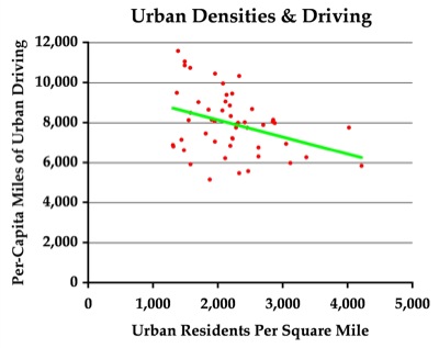
Each red dot represents the urban areas in one of the 50 states; the green line is the average trend. The spread of the dots shows that density is only weakly correlated with driving. The shallow slope of the line shows that, if density does influence driving, large density increases will produce small reductions in driving. Clicking the chart will download the spreadsheet.

Based on the data used to make the chart above, a 1,000-person-per-square-mile increase in urban density is associated with a 395-mile-per-capita reduction in driving. That means if California can increase its densities by 25 percent, from 4,000 to 5,000 people per square mile, it will reduce per-capita urban driving by 5 percent. That assumes, of course, that higher densities are a cause of lower per-capita driving rather than being merely correlated with some other cause such as downtown job densities. To the extent that less driving means more transit ridership, the reduction in greenhouse gas emissions will be slight because we know that, on average, transit emits as much greenhouse gases as passenger cars (though admitted less than SUVs).

Proponents of SB 375 take it for granted that higher densities mean less driving and lower greenhouse gas emissions. But they never mention the costs. Thanks to California’s past land-use planning, the state has the second-least-affordable housing in the nation. (Affordability is slightly worse in Hawaii, the only state that has done growth-management planning longer than California.)

If California’s average urban densities were the same as in the rest of the country — about half its current densities — the state’s housing would be no less affordable than elsewhere. People might drive 800 miles per year more, or about 10 percent more than they drive today, but homebuyers would save about $125 billion or more per year on housing (see page 12).

Californians burn about 18 billion gallons of motor fuel a year, so 10 percent more is 1.8 billion. A gallon of gasoline produces about 20 pounds of carbon dioxide, so 1.8 billion gallons represents about 16 million metric tons of greenhouse gases. If it costs $125 billion to save 16 million tons, the cost per ton is about $7,800. When McKinsey says we can reduce our total greenhouse emissions by a third for no more — and often much less — than $50 a ton, $7,800 a ton is a big waste.

Housing isn’t the only cost of smart growth. SB 375 will impose costs on businesses, increased traffic congestion on shippers and commuters, and higher taxes (or lower public services to make up for the cost of compliance) on all Californians. Needless to say, what has really happened here is that smart-growth advocates jumped on the global warming issue and used it to push their own agenda regardless of the minimal benefits and high costs.

Realistically, California is not likely to increase urban densities by 1,000 people per square mile, or another 25 percent over their current levels. The state has already made housing so unaffordable that people are leaving the state for more affordable lawns elsewhere. All SB 375 will do is increase the costs of living in California still more without saving more than a handful of tons of greenhouse gas emissions.