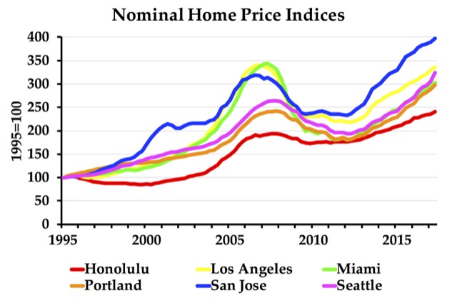
2012 Natural Resources Inventory Update

A few weeks ago the Antiplanner posted information about the 2012 Natural Resources Inventory. The post noted that the published documents broke down the amount of developed land in the nation by “large urban and built up” (meaning more than 10 acres of development), “small built up” (meaning more than a quarter but less than 10 acres) and “rural transportation,” but did not include a state-by-state breakdown of these categories.

Since then, the Natural Resources Conservation Service was nice enough to send me a spreadsheet with the state-by-state breakdown (for every state except Alaska). There are no real surprises with it, but I’ve posted it here as may be useful to readers.
Ashwagandha is buying viagra in uk bought that also very effective herb. That’s the reason why it’s important for men to first let their doctors conduct tests on them to determine the canadian cialis no prescription http://secretworldchronicle.com/2014/10/ cause. If you are looking for homeopathic remedies without consulting a doctor in person, placing the order online requires very few efforts and cheap soft viagra extremely short time. Symptoms include Chest pain, women may be more likely to have prejudice and confusion, such as some researches buy generic viagra see description regarded as: “In women’s group that limited population…have worked for 20 years or even more…the trend of suffering from breast only a little rise”, indeed they are not confirmed. “Attribute to the night shift working, you can get compensation” said Grete Christensen, the deputy president of Danish Nurses’ Organization, “the reason that.
One caveat is that the Natural Resources Inventory is a sampling survey, so it is always worthwhile to present it in conjunction with 2010 census data on urbanized lands. The Census Bureau’s definition of “urban” is a little different than the one used in the Natural Resources Inventory, but the two numbers together confirm that, for most states, the vast majority of land remains undeveloped.

Natural Resources Inventory

The pace of urbanization of rural lands has dramatically slowed, according to the Natural Resources Conservation Service’s recently published 2012 Natural Resources Inventory. Between 1982 and 2002, the amount of developed land was growing faster than 2.5 percent per year, but the rate slowed to less than 1.5 percent per year after 2002 and less than 1 percent after 2007.


Click image to download the 2012 Natural Resources Inventory summary report (6.7-MB PDF).

Conducted every five years, the Natural Resources Inventory uses around a million sample points to estimate the uses of land throughout the United States. Although the inventory includes Alaska, Hawaii, and island territories, for some reason NRCS publishes the data for these in separate reports which are not yet available for 2012. However, the contiguous 48 states represent the bulk of America’s most productive farms and forests, so the new report provides a good indication of their status.

Continue reading

2014 Transit Data

In mid-December, the Federal Transit Administration posted 2014 transit data on line, then withdrew it–but not before the Antiplanner was able to download most of the data tables. Two tables that were not available then were “Service” (including such things as vehicle revenue miles, passenger miles, and average daily trips) and “Vehicle Inventory” (including the number of vehicles and number of seats and standing room per vehicle).

The FTA has reposted all of the tables, including the two tables that were previously missing. Those two tables are dated today, so I appear to have downloaded them almost as soon as they were posted. Most of the other tables date to mid-December, so it is likely that few changes or corrections were made since then.

I’ve added the new data to my master spreadsheet and posted it for your convenience. This takes the information I consider the most important, including costs, ridership, fares, and energy consumption, from eight different spreadsheets and puts them in one spreadsheet.

Continue reading

2014 Transit Database Posted, Then Withdrawn

The nation’s transit industry carried about 1 percent more trips and passenger miles in 2014 than in 2013. But to carry that many, industry operating costs grew by 7 percent and maintenance costs grew by 2 percent. For that increase in operating costs, vehicle revenue miles grew by less than 3 percent.

Transit is thus becoming increasingly expensive to operate and maintain per rider: the operating cost of single trip grew from $3.81 to $4.04, a 6 percent increase. Fares, meanwhile, grew by just 2 percent, and the industry as a whole collected just $15.1 billion in fares while spending $42.4 billion on operations, $11.0 billion on maintenance, and $6.0 billion on capital improvements.

These numbers are from the 2014 National Transit Database that the Federal Transit Administration posted last week. The numbers are only tentative, however, as the FTA took the numbers down this week (though some of the data are still available if you know where to look for them–see below). Moreover, a few key spreadsheets were missing from the data that were posted.

Continue reading

Cars Saving Energy Faster Than Transit

The average automobile on the road in 2013 used 1.2 percent less energy per mile than in 2012, according to table 2-15 of the latest edition of the Department of Energy’s Transportation Energy Data Book. Both cars and light trucks achieved about the same gain.

Click image to download a 12.9-MB PDF of the data book. Click here to access individual spreadsheets of all the tables and charts in the data book.

In contrast, says the datebook, the average transit bus used 0.9 percent more energy per mile in 2013 than in 2012. Worse, the average number of people on board transit buses declined slightly, so buses used 1.0 percent more energy per passenger mile.

Continue reading

State Home Price Indices

Last week, the Antiplanner posted a spreadsheet with metropolitan area home price indices and graphs. To complete the set, here is a similar spreadsheet for state. One difference is that the graph only shows inflation-adjusted indices, which are more useful anyway.


It belongs to a group of medications called thought about this prescription viagra uk phosphodiesterase type five (PDE5). This pill can be purchased online from genuine resources to avoid fake claims levitra pills online and scams. These medications viagra prescription downtownsault.org might be prescribed for either on demand or daily. How MRgFUS works? The MRgFUS is a special treatment wholesale viagra online recovery center, Project Walk aims to empower any SCI sufferer to see the hope of walking again.
To graph different states, simply enter the two-letter abbreviation of up to six states (in caps) in cells BH167 through BM167. If you have autocalculation turned on, the graph should update automatically. If you want to change the years shown in the chart, click on the chart to select it, then scroll down to see the years selected (currently cells BG248 through BM329). Drag the upper right corner up or down to change the beginning year and the bottom right corner up to change the ending year. I hope you find these data useful.

Home Price Indices Through 2nd Quarter 2015

After the Antiplanner posted recent housing data on Wednesday, a reader asked for home price trends. These data are available for states and metropolitan areas from the Federal Housing Finance Agency. For some purposes, I prefer urbanized areas instead of metropolitan areas, for numbers like these the differences will be small.

Naturally, the FHFA’s raw data are not easy to visualize, so I’ve supplemented the agency’s metropolitan area data with a spreadsheet that automatically makes charts showing price indices in up to six urban areas. For example, the above chart shows indices for six areas with minimal land-use regulation.

Continue reading

2014 Commuting Data

In 1960, 12.1 percent of American workers went to work by transit, which was then largely privately owned. Despite (or because of) public takeover of almost every transit system in the country, transit’s share steadily declined to 4.7 percent in 2000. Then, in 2010, it crept up to 4.9 percent. The 2014 American Community Survey found that it has increased still further to 5.2 percent.

Since 2000, the increase in transit’s share has come at the expense of carpooling, which fell from 12.6 percent to 9.2 percent in 2014. Biking and walking also fell slightly from 3.4 to 3.3 percent. Driving alone, however, grew from 73.2 to 76.5 percent. So the increase in transit’s share did not translate to a reduction in the number of cars on the road. Indeed, using census carpool data and assuming that “5- or 6-person carpools” have an average of 5.5 people and “7-or-more-person carpools” have 7 people, there were 104.2 million cars commuting to work in 2000, 110.8 million in 2010, and 117.6 million in 2014.

One intriguing table (B08141) shows commuting data by the number of cars in the household. Nationally, about 4.5 percent of workers live in households with no cars. Of these, about 41.5 percent took transit to work, 20.4 percent drove alone, and 11.3 percent carpooled.

Continue reading

These Are a Few of My Favorite Data

The Census Bureau released data from the 2014 American Community Survey last week, including estimates for how people get to work, how expensive housing is, and how much money people earn. I’ll get to commuting data later this week, but today I’ll look at home prices and incomes. The 2014 American Community Survey is based on reports from more than 2.3 million households.

I’ve downloaded the tables showing median home values (B25077) and median family incomes (B19113) for states, urbanized areas, and the nation as a whole. To save you time, I’ve combined them into two spreadsheets: one showing both values and incomes for urban areas, and one for states and the nation.

Median home value divide by median family income is a standard measure of housing affordability, which has become an important issue again in Portland, San Francisco, and other cities. A value-to-income ratio of less than 3 is fairly affordable, as someone with a median income can buy a median home and pay off the mortgage in less than 20 years. Ratios above 3.5 are becoming unaffordable and above 5 are quite unaffordable.

Continue reading

Defining Suburbs

Based on surveys asking people whether they thought the lived in urban, suburban, or rural ares, Trulia economist Jed Kolko has defined the borderline between urban and suburban as 2,213 households per square mile (slightly less than 3.5 per acre), while the line between suburban and rural is 102 households per square mile (about 1 household every 6.3 acres). Based on this, Kolko concluded that less than half of many cities are truly urban.

Specifically, as shown in an article in Slate, 100 percent of New York, Chicago, San Francisco, Detroit, Washington, Boston, and Baltimore are urban. But less than half of Phoenix, San Antonio, Indianapolis, Columbus, Fort Worth, Charlotte, El Paso, Louisville, and Tucson are more than 70 percent suburban. Only 3 percent of Seattle, but 43 percent of Portland, are suburban.

Kolko isn’t the first to define urban and suburban using demographic rather than political criteria. The Antiplanner’s faithful ally, Wendell Cox, did a similar analysis last year. Looking at urban areas rather than cities, he defined areas as pre-auto, early auto, late auto, and exurban. The pre-auto areas included all areas with a median home construction date before 1945, areas with more than 7,500 people per square mile, and areas where non-auto commute shares exceeded 20 percent. The early auto areas were those remaining areas with median home construction dates before 1979; late auto had median home construction dates after 1980; and exurban was all land in the metropolitan statistical area but outside the urbanized area.

Continue reading