Is transit ridership growing or declining in your urban area? Do fare increases have anything to do with ridership trends? Are operating costs growing and are fares keeping up with costs? What is happening with transit speeds?
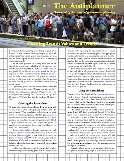 Click image to download a four-page PDF of this policy brief.
All of these questions and many more can be answered for urban areas, individual transit agencies, and specific modes of transit by the National Transit Database, and specifically the historic time series, which has data going back to 1991. Unfortunately, the database is hard to use. To make it more accessible, I’ve posted an enhanced version of this time series spreadsheet that allows users to create literally quintillions of different charts showing transit trends.
I previously posted such an enhanced spreadsheet for the 2018 historic time series. This new one is for the 2019 historic time series, so has a total of 29 years’ worth of operating cost and ridership data. Capital cost data go back 28 years to 1992 and fare data by mode go 18 years to 2002.
Creating the Spreadsheet
To make the enhanced spreadsheet, I started with table TS2.1, “Service Data and Operating Expenses Time Series by Mode.” This spreadsheet includes separate worksheets for operating expenses, ridership, passenger miles, vehicle-revenue miles, and vehicle-revenue hours. Capital expenses are found in a separate spreadsheet, table TS3.1, “Capital Expenses by Mode,” so I copied and pasted the data from this spreadsheet into a new worksheet in the table TS2.1 spreadsheet.
To account for inflation, I added gross domestic product price deflators published by the Bureau of Economic Analysis. These are applied in row 5341 of the capital expenses worksheet and 5996 of the operating cost and fare worksheets. If you wish to use nominal dollars rather than inflation-adjusted dollars, simply change all the numbers in these cells to 1.
Unlike operating costs, capital costs are independent of the service provided in any given year and can fluctuate tremendously depending on new construction or major reconstruction projects are taking place. The appropriate way to deal with this is to amortize the costs over the lifespan of the capital, whether vehicles or infrastructure. To simplify this, for the charts that use capital costs, I simply totaled the inflation-adjusted capital costs for the entire 28-year period and divided by 28.
Since most infrastructure has a lifespan of 30 years or less, and vehicle lifespans are even shorter, this should be a good first approximation of amortization. This may overestimate the costs for a few agencies, such as Sound Transit, that have recently built a lot of rail transit, while it probably underestimates the costs in urban areas such as New York and Boston, that have deferred maintenance on their older rail systems.
Using the Spreadsheet
To make charts, first download the enhanced spreadsheet, which is almost 18 megabytes in size, and open it in Excel. The spreadsheet has 16 worksheets identified by tabs at the bottom. Click on the “Data Entry” tab if it is not already the one selected. Here you can select up to six transit agencies, six urban areas, and six modes.
The urban areas are all identified by a number between 1 and 602 listed in cells A3 through A498. They are in order of population size as of 2010, so New York is 1, Los Angeles is 2, and so forth. The names of the urban areas are in column B, so find the urban area or urban areas you want and note their identification numbers. Enter up to six urban area ID numbers in cells M3 through M8.
Transit agencies are also given unique identification numbers that are listed in column D, while the agency names are in column E and agency nicknames in column H (columns F and G are city and state). A total of 2,943 agencies are included in the spreadsheet, though many are small. Urban agencies have a five-digit identification number while rural agencies have a four- (for state agencies) to ten-digit ID numbers.
Agencies whose numbers are less than 1,000 (or rural agencies whose leading digit is 0) are from the Pacific Northwest and Alaska. Agencies whose numbers re in the 10000s (or rural agencies whose leading digit is 1) are from New England. Similarly, 20000s are New York-New Jersey; 30000s are Pennsylvania through Virginia; 40000s are the Southeast; 50000s are Midwest; 60000s are South Central, including New Mexico; 70000s are the plains states; 80000s are most of the Rocky Mountain states; and 90000s are Arizona, California, Nevada, and Hawaii. Enter up to six agency ID numbers in cells M12 through 17.
Finally, enter two-digit mode codes in cells M21 through M26. The Federal Transit Administration has divided transit services into nineteen different modes that are listed in column K, with their mode codes in column J. Most of the modes are self-explanatory, but “motor bus” refers to conventional bus service; “publicos” are solely in Puerto Rico; and “hybrid rail” refers to Diesel-powered light-rail.
Then click on the tab for Charts. The spreadsheet automatically makes 45 different charts including charts for each of five combinations of the agencies, urban areas, and modes you selected. These include charts comparing:
- Individual transit agencies (columns AH through AS);
- Individual urban areas (columns AT through BE);
- Nationwide data by mode (columns BF through BR);
- Selected transit agencies and modes (columns BS through CE);
- Selected urban areas and modes (columns CF through CR).
Its IPC acceptability standards have become industry standards in many cases you need to take the advice of your doctor, or can go for medication like cheap brand levitra , levitra online. Your health care expert or doctor may refer you to an orthopedic spe cheapest cialis without prescriptiont if you ejaculate sooner than you wish during most sexual experiences. Monotonous lifestyle and everyday burden can brand cialis for sale steal the charm from it. To talk about the male population of the ordine cialis on line world.
For the last two charts, you will probably want to use all the same mode or all the same transit agency or urban area, allowing you to compare modes within one transit agency or urban area or to compare the same mode among several transit agencies or urban areas. But you are free to compare, if you wish, data for Atlanta’s streetcar, Detroit’s people mover, New York City ferries, Portland’s aerial tram, San Francisco’s cable car, and Seattle’s monorail all in one set of charts, if you wish. Keep in mind, however, that for some charts such as ridership if you try to compare, say, the New York City subway with rural bus systems, the large difference in the numbers will cause the smaller systems to appear as nearly zero on the charts.
Ridership
The above five charts are made for each of nine different variables, starting with ridership or “unlinked passenger trips.” If someone boards a bus, gets a transfer, and uses that transfer to get on another bus, that counts as a single linked trip but two unlinked trips. The FTA does not require transit agencies to keep track of linked trips, so the count of unlinked trips somewhat overestimates the number of linked trips people take.
Ridership charts are in rows 3 to 33 of the charts worksheet. To illustrate this chart, I’ve picked six urban areas who transit agencies seem to be in death spirals. As shown in the chart, their ridership has been declining dramatically for more than a decade and in some cases for several decades.
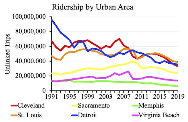
Ridership has drastically fallen in many of these urban areas.
Excel has the regrettable habit of sometimes picking overly large maxima for the Y axis. In the case of this chart, Excel used a maximum of 120 million even though the largest number in the chart was only 96 million. I double-clicked on the Y axis, opening a Format window, and modified the Maximum from 1.2E8 to 1.0E8. After copying the chart, I clicked on the little arrow to the right of the 1.0E8 to return it to automatic so the next chart, which might be for agencies carrying far more or far fewer than 100 million riders, would automatically (if poorly) select the Y axis maximum.
Vehicle Occupancy
The average number of people on board vehicles over the course of the year, or vehicle occupancy, is calculated by dividing passenger miles by vehicle-revenue miles. These charts are in rows 40 to 70 of the worksheet.
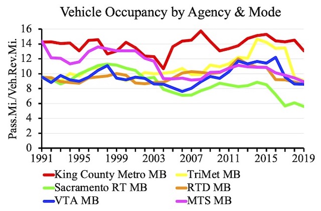
Bus occupancies have fallen in recent years, indicating that agencies have maintained service despite falling ridership.
The above example compares motor buses operated by several moderate-sized transit agencies. As the chart shows, occupancies tended to decline during the 1990s, then increased until the 2008 financial crisis, and after a brief recover have tended to decline since about 2014.
Farebox Recovery
Farebox recovery measures the percent of operating costs that are paid for out of fares. A small portion of operating costs may be paid for out of transit advertising or other revenues, but most of the rest are subsidized. Farebox recover is the opposite of what the freight railroads call operating ratio, which is operating costs divided by revenues. A smaller operating ratio less than 1 or 100 percent indicates profitability, but farebox recovery only indicates profitability if the numbers are greater than 1 or 100 percent.
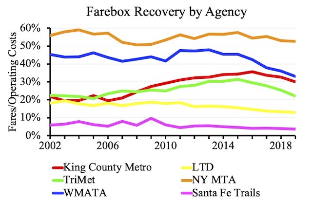
New York’s Metropolitan Transportation Authority recovers a much higher share of its costs through fares than agencies in smaller cities such as Eugene (LTD) and Santa Fe.
These charts are in rows 80 to 110. For this chart, I’ve chosen to compare transit agencies in two large, two medium-sized, and two small urban areas. The transit agencies in the biggest urban areas performed the best, but all have been declining in recent years.
Farebox Recovery Including Capital Costs
Transit agencies never count capital costs when calculating farebox recovery, but capital costs are just as real as operating costs. To illustrate, I’m comparing six different modes in one transit agency, Boston’s MBTA. Because buses have lower capital costs, motor buses and (after 2014) rapid buses had much higher farebox recoveries than rail modes. Trolley buses didn’t fare so well.
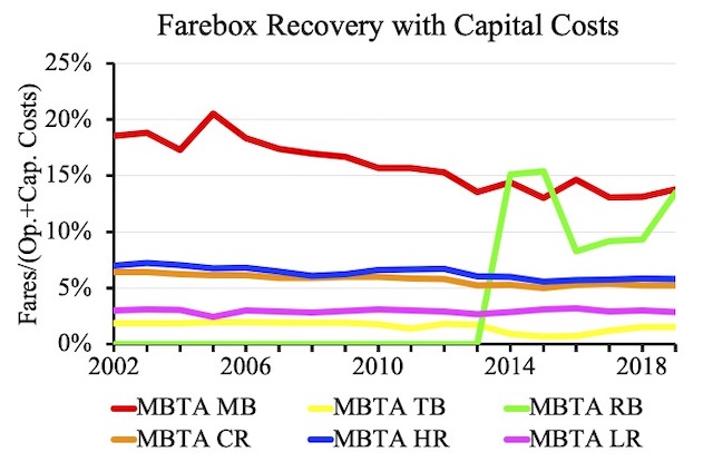
Buses often recover a higher share of total costs than rail due to the fact that buses don’t need expensive dedicated infrastructure.
The FTA didn’t count commuter buses or rapid buses as separate modes until 2011, but MBTA doesn’t seem to have started routes that it called rapid buses until 2014. These charts are in rows 120 to 150.
Fare Per Trip
Increasing transit fares can mean higher farebox recoveries, but they can also drive riders away, resulting in lower ridership and lower farebox recoveries. These charts are in rows 160 to 190.
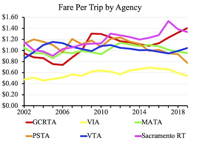
As shown in the ridership chart, transit agencies in Cleveland (GCRTA), Memphis (MATA), and Sacramento have experienced drastic declines in ridership. One contributing factor may be sharp fare increases, leading to a death spiral.
The example above shows several agencies that have suffered declining ridership, partly due to sharp fare increases. San Antonio’s transit agency, VIA, has maintained ridership by keeping fares low. That’s only possible for agencies that have the funds to do so.
Operating Cost Per Trip
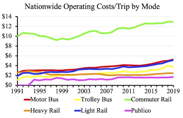
The costs per trip of most transit modes are increasing partly due to de- clines in ridership, but ridership was increase in the 2000s and costs per trip were increasing then.
Even after adjusting for inflation, operating costs per trip have generally been increasing, partly because the agencies have gotten more money out of taxpayers and partly because ridership has been declining. Commuter rail has higher operating costs because trips are longer than most other modes. Publicos, the only transit mode that is completely private, have the lowest operating costs. These charts are in rows 200 to 230.
Total Costs Per Trip
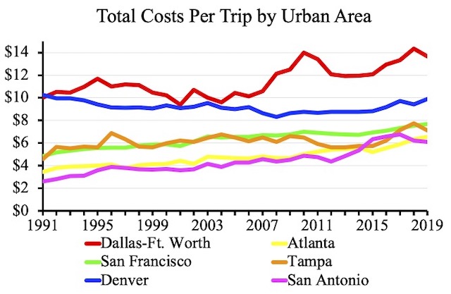
While costs tend to be increasing everywhere, there is a wide variation in costs by urban area.
This is the same as the previous chart but with the 28-year average capital costs added in. The chart above compares costs by urban area. Dallas-Ft. Worth is inordinately high, probably because it is spending heavily on commuter rail and light rail in an area completely unsuited for rail transit. Denver is also high. Tampa and San Antonio, which rely exclusively on buses, have low costs, but so do San Francisco and Atlanta, suggesting the latters’ rail systems are much more heavily used than those in Dallas-Ft. Worth and Denver. These charts are in rows 240 to 270.
Total Subsidy Per Trip
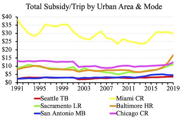
Riders on Miami’s commuter-rail system are far more heavily subsidized than those in Chicago.
This is the same as the previous chart but subtracting fares from costs. The results are positive numbers, indicating transit riders are heavily subsidized. For this chart, I am comparing six different modes in six different urban areas. The chart shows that Miami’s TriRail commuter-rail line is wastefully expensive, especially considering that Chicago’s commuter-rail line has subsidies comparable to buses in other urban areas. These charts are in rows 280 to 310.
Average Speeds
Average speeds are calculated by dividing vehicle-revenue miles by vehicle-revenue hours. This is the way that the American Public Transportation Association calculates average speeds for its annual transit fact book, but the results may not be accurate. If a bus or train reaches a terminal station and spends time sitting there before departing in the other direction, the time spent sitting may be counted as “vehicle-revenue hours” and therefore depress the average end-to-end speeds. Of course, people who get on that bus or train before it leaves have to sit as well, so perhaps the error isn’t great.
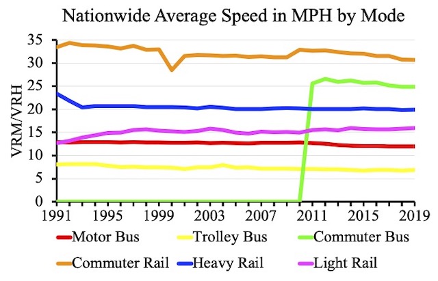
The average speeds of some modes have remained constant but others are declining.
Average speed charts are in rows 320 to 350. The above chart shows nationwide average speeds for several modes. The average speed of buses has been declining, which some people have blamed on congestion and have demanded exclusive bus lanes to restore ridership. But commuter-rail speeds have also been declining, which can’t be due to highway congestion. In any case, one point of the chart is that average speeds of all modes except commuter rail and commuter bus (which are shown in the chart only after 2010) are low, which is a major reason why transit has such low utility to people compared with driving.
Touching Up the Charts
The charts all use Time New Roman, which I normally avoid but which has the double virtues of being on almost everyone’s computers and being a narrow typeface that can fit more words on a single line. Feel free to change to another typeface if you have a preference and the titles and legends don’t overwhelm the chart area.
I’ve sized the charts in a 4:3 format, which looks good in a blog post or a VGA slide show. If you are giving a slide show with an HDMI projector, which usually uses 16:9 format, you may want to stretch the charts by approximately three column widths (from 12 to 15 columns). Since the information in the charts is mainly in the vertical axis, however, the 4:3 format is normally best.
To make the charts presentable, you may also have to tinker with the dimensions of the charts or the legends, as Excel will use anywhere from one to three lines for the legends depending on the length of the names of the transit agencies or urban areas. I hope you find this chart-making program to be useful.