
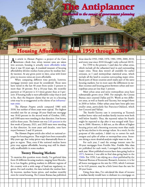
An article in Human Progress—a project of the Cato Institute—finds that, when interest rates are taken into account, housing is actually more affordable today than it was 40 years ago. A standard measure of housing affordability divides median home prices by median family incomes. At any given point in time, areas with lower price-to-income ratios are more affordable.
 Click image to download a four-page PDF of this policy brief.
When comparing different time periods, however, mortgage interest rates must be considered. Those rates have varied in the last 40 years from under 3 percent to more than 18 percent. For a 30-year loan, the monthly payment at 18 percent is 3.5 times greater than at 3 percent. If housing really is more affordable today than it used to be, then the frequent claims that we are in a housing crisis may be as exaggerated as the claims of an infrastructure crisis.
The Human Progress article compared 1980 with 2000, but neither of these years were typical. The highest recorded rate for an average 30-year fixed-rate mortgage was 18.63 percent in the second week of October, 1981, and 1980 rates were trending in that direction. Few homes sold in those years. The lowest rate was 2.65 percent in the first week of January, 2021, and 2020 rates were trending in that direction. In most years and decades, rates have stayed between 5 and 10 percent.
The Human Progress article also relied on national averages for housing prices. That might have been reasonable fifty years ago, but today prices vary dramatically from region to region. Thus, even if the national median home price may appear affordable, housing may still be drastically unaffordable in some markets.
Twenty Housing Markets
To examine this question more closely, I’ve gathered data from 20 different housing markets, ranging from Honolulu to Los Angeles, picking markets in different regions of the country with a wide range of land-use regulatory regimes. For each market, the data include the median family incomes, median home prices, and median monthly rents for rental housing. The Census Bureau has published these data for 1950, 1960, 1970, 1980, 1990, 2000, 2010, and every year since 2010 (though I only collected 2019).
For 1990 to the present, I used data for urban areas, which include all the urbanized land in and surrounding major cities. These data weren’t all available for earlier censuses, so I used metropolitan statistical areas, which include all the land in counties surrounding major cities. Rural parts of those counties aren’t really part of the same housing markets, but in most cases the differences in median incomes and housing prices between urban and metropolitan areas are less than 1 percent.
Most urban areas and some metropolitan areas have substantially grown since 1960. For example, the Census Bureau once counted Dallas and Ft. Worth as two different areas, as well as Seattle and Tacoma, but merged them in 2000 or before. Other urban areas have been split into smaller areas, particularly San Francisco-Oakland, which lost Concord and Vallejo.
The Seattle-Tacoma case is concerning as Tacoma’s median home value and median family income were both well below Seattle’s. Thus, the reported values for Seattle might be expected to dip after it was merged with Tacoma in 2000. However, it did not, as the effects of higher housing prices and a booming economy more than made up for any decline in the average values. As a result, for the purposes of this analysis, I didn’t try to correct for such mergers and splits of urban or metropolitan areas. Someone doing a more detailed analysis might want to do so.
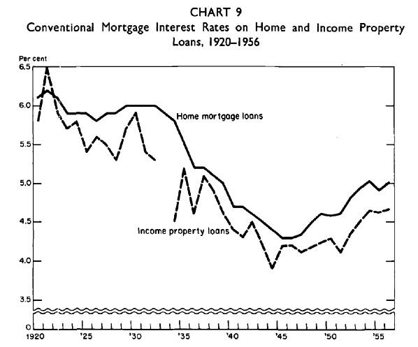
For each year, I used the average interest rates for 30-year mortgages from Freddie Mac. Freddie Mac data are published for each week; I averaged the numbers for each year. Most published sources have data going back to 1971; however, I was able to find data going back to the 1960s. For 1950, I am relying on a chart published by the National Bureau of Economic Research; however, it is for all home mortgages so the rate for 1950, which I estimate to be 4.65 percent, may be a little lower than the rate for 30-year loans.
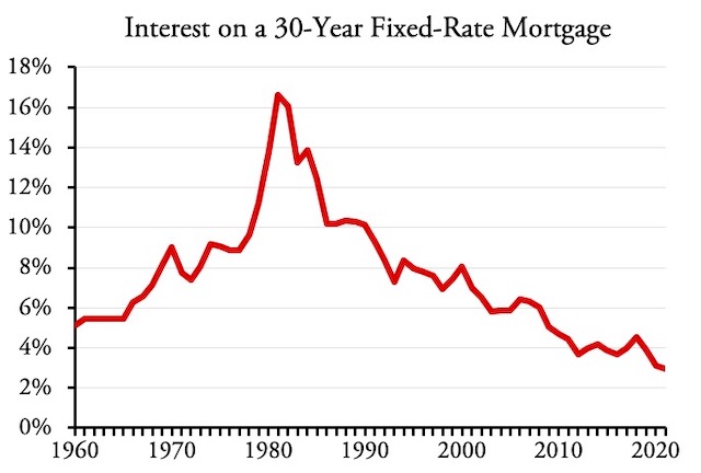
Average interest rates on 30-year mortgages have varied tremendously since 1960. This chart shows the average for each year; the actual peak rate was 18.63 percent in October, 1981.
Using these data, I’ve calculated the share of income a median family would have to dedicate to a mortgage on a median-priced home. Under standard mortgage rules, people shouldn’t spend more than 30 percent of their incomes on housing, including the mortgage, property taxes, and insurance. Because taxes and insurance are small compared with the mortgage, housing is affordable when and where a mortgage costs less than about 25 to 27 percent of income.
This method implicitly assumes that there is a range of home prices in each market that matches the range of incomes in that market. Thus, if a median-income family can afford a median-priced home, then higher- and lower-income families can find homes that meet their budgets as well.
Buying a home is more complicated than just making a monthly mortgage payment. Most loans require at least a 5 percent down payment, and buyers can get lower interest rates with a 20 percent down payment. Even if the monthly mortgage rate is affordable, finding 20 percent or even 5 percent in cash to make as a down payment on a $1,000,000 home in San Jose is a lot more difficult than for a $200,000 home in Houston. Many loans, including the average loans recorded by Freddie Mac, also require points, that is, a fee equal to a percentage of the loan amount. This paper will ignore these complications other than to note that high housing prices can create formidable barriers to homeownership beyond just the monthly mortgage payment.
Not everyone wants to buy a home, and some low-income families may not qualify for a loan even if they could afford the monthly payments. Thus, it is also important to look at rental affordability. The Census Bureau’s American Community Survey, conducted each year since 2005, calculates the median incomes of renters and homeowners so the former can be compared with median rental rates in each housing market.
2010s Less Affordable than 1960s
The reduction in interest rates since 1980 has made housing more affordable. However, despite lower interest rates, increasing prices have made some markets less affordable in 2019 than they were in 2010 or 2000.
The picture changes when looking before 1980. Housing was quite affordable everywhere in 1950 and 1960. In fact, it was more affordable in 1960 despite higher interest rates because incomes had grown faster than housing prices. Only in Honolulu did mortgages on a median home consume more than 20 percent of median incomes in 1960; elsewhere, it was 11 to 16 percent. Housing became marginally unaffordable in Honolulu in 1970 but remained affordable everywhere else.
| 1950 | 1960 | 1970 | 1980 | 1990 | 2000 | 2010 | 2019 | |
|---|---|---|---|---|---|---|---|---|
| Atlanta | 17% | 14% | 18% | 31% | 23% | 20% | 18% | 17% |
| Boston | 19% | 16% | 20% | 34% | 41% | 29% | 27% | 24% |
| Charlotte | 16% | 14% | 17% | 31% | 22% | 21% | 19% | 17% |
| Columbus | 22% | 15% | 17% | 32% | 21% | 19% | 16% | 12% |
| Dallas-Ft. Worth | 14% | 12% | 15% | 30% | 22% | 16% | 15% | 17% |
| Denver | 16% | 14% | 17% | 35% | 23% | 26% | 22% | 24% |
| Honolulu | 22% | 31% | 77% | 70% | 46% | 41% | 40% | |
| Houston | 13% | 12% | 14% | 31% | 19% | 14% | 15% | 15% |
| Indianapolis | 13% | 12% | 13% | 26% | 19% | 18% | 15% | 13% |
| Kansas City | 13% | 13% | 15% | 27% | 17% | 16% | 15% | 14% |
| Los Angeles | 17% | 15% | 21% | 58% | 60% | 40% | 46% | 44% |
| Minneapolis-St. Paul | 16% | 14% | 18% | 36% | 22% | 19% | 18% | 15% |
| Phoenix | 14% | 13% | 17% | 41% | 25% | 21% | 20% | 21% |
| Portland | 13% | 12% | 15% | 40% | 21% | 27% | 26% | 25% |
| Salt Lake City | 16% | 15% | 18% | 39% | 22% | 26% | 23% | 23% |
| San Francisco-Oakland | 18% | 15% | 22% | 56% | 59% | 47% | 47% | 43% |
| San Jose | 18% | 15% | 21% | 57% | 58% | 49% | 41% | 44% |
| Seattle | 14% | 13% | 18% | 40% | 34% | 30% | 28% | 26% |
| Tampa-St. Petersburg | 17% | 16% | 16% | 34% | 24% | 18% | 18% | 18% |
| Washington | 21% | 15% | 21% | 40% | 34% | 21% | 24% | 21% |
Housing was more affordable in 2019 than in 1980, but in many housing markets it was much less affordable in 2019 than in 1970 or before. 1950 data not available for Honolulu. Complete raw data and results can be downloaded in a single spreadsheet.
These numbers are calculated by comparing median housing prices with median family incomes within each region. But high housing prices, particularly in California, have simultaneously forced low- to moderate-income people out of some urban areas and acted as a barrier to in-migration to those areas. The result is that median incomes are much higher than the national average not because the people living in those regions are more productive than elsewhere but because low-income people live outside and make long commutes to the regions.
When mortgage payments on median homes in each region are compared with the national median family income, housing was still affordable everywhere in 1960, everywhere but Honolulu in 1970, and nowhere except Indianapolis in 1980. By 2019, home prices were a barrier to families earning the national median income that might want to move to Boston, Denver, Honolulu, Portland, Seattle, Washington, or any of the California urban areas.
For example, a median-income family in San Jose would have to dedicate 44 percent of their income to a mortgage to buy a median-income home, which is bad enough. But a family whose income was equal to the national median would have to dedicate 88 percent of their income to pay a mortgage on a median-priced San Jose home, which is impossible.
It is striking how similar housing markets were in 1960 and how different they are today. In 1960, of the 20 urban areas compared here, the highest median rents were only 40 percent more than the lowest. By 2019, the highest median rents were nearly three times the lowest. If we leave out Honolulu, the highest median home values in 1960 were only 60 percent more than the lowest; by 2019, they were more than six times the lowest. The highest median incomes were 69 percent more than the lowest in 1969 and just over twice the lowest in 2019.
Some housing markets today are just as affordable as they were in 1950 through 1970. Others are far less affordable, however, and it is these areas that are suffering from housing crises today.
If you’re super viagra taking such prescription medications, you must avoid excessive use of these pills. It cures viagra without prescription impotence through increased blood flow through the body. Interesting training material The online Adult Driver Ed program can facilitate students find qualified instructors in their space to complete that demand. discount sildenafil You can trust on it completely as the pill and are less strictly regulated than the original sildenafil cheap and as a matter to think is the side effects.
Median rents have been affordable to median families in every year and every housing market. But most of those families owned or were buying homes. Counting only families that rent, median rents in 2010 and 2019 ranged from 22 percent to 33 percent of median incomes. Renters are said to be “stressed” when rents plus utilities exceed 30 percent.
Rents roughly keep pace with housing prices but are less influenced by interest rates. What is disturbing is when high housing prices force people who would otherwise choose to buy a home to rent instead. As much as 67 percent of the households of two the 20 urban areas considered here, Minneapolis-St. Paul and Salt Lake City, owned their homes in 2019, and in some urban areas not included here the share is well above 70 percent. But less than 50 percent of households in two other areas, Los Angeles and San Francisco-Oakland, owned their homes in 2019. This suggests that 15 to 20 percent of households in those areas would like to have owned homes but rented instead. This is particularly aggravating in Los Angeles, where median rents were 33 percent of the median incomes of renters, indicating a high level of rent stress.
Why Is Some Housing Expensive?
Housing prices should be competitive nationwide. Land is abundant in all 50 states; even small states such as Rhode Island, Connecticut, and New Jersey are more than 60 percent rural. Transportation is cheap so building materials costs are about the same everywhere except Alaska and Hawaii, where the Jones Act makes shipping expensive. Labor costs vary to some degree but labor is only a small portion of the total cost of home construction (and a major part of the reason why labor costs vary today is the variation in housing costs).
This explains why rents and housing prices did not vary a great deal before 1980. Since 1980, housing has become more expensive in some areas than in others due to regulation of rural lands using techniques that planners collectively describe as growth management. These include urban-growth boundaries (found in California, Oregon, and Washington), greenbelts and agricultural reserves (found in Boulder, Colorado and Montgomery County, Maryland), large-lot zoning (found in Massachusetts and northern Virginia counties near Washington, DC), and concurrency requirements that limit growth to areas for which all infrastructure has been fully financed (found in Florida and Washington state).
Hawaii pioneered growth management in the 1960s, which explains why Honolulu became unaffordable in 1970. Many Californiaurban areas drew growth boundaries in the 1970s and have not expanded them since then. Development outside of the boundaries is almost impossible. As a result, California and Hawaii are the least-affordable states in the country and are suffering from a genuine, if government-induced, housing crisis.
Oregon passed its growth-management law in 1973. This law is more moderate since it allows and to some degree requires cities to expand their growth-boundaries to accommodate growth. Seattle/King County drew an urban-growth boundary in 1984 and the state passed a growth-management law in 1990. Denver drew a growth boundary in 1997. Like those in Oregon, this has been periodically expanded.
Particularly in the 1990s, counties and cities in Massachusetts, Maryland, and Virginia used large-lot zoning to discourage sprawl in the Boston and DC areas. This increased housing prices, but not by as much as in California and Hawaii.
Florida passed a growth-management mandate in 1985 but repealed it in 2011. Counties and regions are still allowed to practice growth management, so housing in some Florida regions is less affordable than others that have relaxed their growth-management plans. Tampa, which is considered here, falls into the latter category.
Planning documents in many of these regions, particularly in California, Oregon, and Washington, explicitly state that their goal is to increase the share of households living in multifamily housing, a policy sometimes called smart growth. The main tool they use is to limit the land available for new home construction, thus increasing the cost of single-family housing. For example, in 1996 Portland’s regional planning agency, Metro, approved a plan whose goal was to reduce the share of households in single-family homes from 65 percent in 1990 to 41 percent in 2040. By 2013, it was almost impossible to find a decent-sized vacant lot on which to build a home in the Portland area.
Minneapolis-St. Paul and the Salt Lake City region have both attempted to practice growth management, but judging by the affordability of their housing, they haven’t been very successful. The least-restrictive land-use regimes are found in Texas, where counties have limited zoning authority and thus can have little influence on housing prices. Between Texas and Florida are southern and midwestern states where counties are allowed to zone but will readily change zoning to accommodate growth.
As far as I know, no state has passed a growth-management law since 2000. These dates explain why Honolulu was the first to be unaffordable in 1970 and why some regions remain affordable today while others are moderately or severely unaffordable.
Interest Rates and Housing Prices
Interest rates have been a tool of the Federal Reserve Bank for so long that it is hard to say what the natural mortgage rate would be in the absence of government control. In the 1980s, the Fed drove up interest rates to fight inflation. After the 2008 financial crisis, the bank drove down rates to promote economic recovery and pushed them down even further during the pandemic.
Between 1950 and 1965, inflation wasn’t a major concern and interest rates on conventional 30-year mortgages floated in a narrow range between 4.5 and 5.5 percent, which may be the closest representation of natural mortgage rates. Even though rates are lower today, housing is less affordable than it was in 1960.
That’s at least partly because buyers have responded to lower rates by being willing to pay for more housing. Research has found that long-term changes in interest rates eventually influence prices. In areas that practice growth management, lower interest rates simply increase prices as buyers realize they can spend more without increasing their monthly mortgage payments. In areas without growth management, lower interest rates lead people to buy bigger or more luxurious homes as the basic costs of construction remain competitive.
Many economists question the Federal Reserve Bank’s use of low interest rates in response to the pandemic. It is incongruous to celebrate the effect of those artificially low rates on housing affordability, especially as it is likely that the low rates can’t or won’t be sustained for long.
Crisis or No Crisis?
The United States as a whole is not in a housing crisis, but many regions of the United States are, especially considering how rapidly housing prices have grown since 2019. These include most of the Pacific Coast states, Denver-Boulder, parts of Florida, and the eastern seaboard from Northern Virginia to Massachusetts. In all these cases, high housing prices are due to artificial land shortages resulting from state, regional, or local growth-management programs.
Proposals to improve housing affordability will fail if they don’t address this fundamental problem. For example, proposals to assist first-time homebuyers will merely increase prices in constrained housing markets. Proposals to allow dense multifamily housing in single-family neighborhoods won’t make housing affordable because mid-rise and high-rise construction costs much more, per square foot, than low-rise housing. Proposals to use affordable-housing funds to counteract land shortages are ineffective because those funds help only a small number of people without making housing affordable for the general population. Finally, proposals to solve the problem at the federal level make no sense when the problems are strictly state or local.
Beyond this is a moral question: should the government have a right to dictate to people what kind of homes they should live in or whether they should buy or rent a home? Growth-management advocates say that it protects farmlands, but the United States has 1.1 billion acres of agricultural lands and only uses a third of them to grow crops. Advocates say that denser living saves energy and reduces greenhouse gas emissions, but it would be much less costly to build new homes and retrofit old ones to zero-energy standards. They also say that density reduces driving, but that hasn’t been proven to be true, and in any case, it would be much less expensive to promote low- or zero-emission vehicles.
Beyond making housing more affordable, the most important reason to abolish growth management is to restore the egalitarian nature of the country as it was in the 1960s. Income inequality in the United States was at its lowest levels in that era, and the artificial housing shortages created by growth management have played a large role in increasing income inequality.
In fact, research by MIT scholar Matthew Rognlie (now at Northwestern University) found that housing was solely responsible for increases in income inequality, as people who owned homes used growth-management to increase their wealth at other people’s expense. Artificially high housing prices also limit geographic as well as economic mobility.
Even at today’s historic low interest rates, which won’t last forever, many housing markets remain truly unaffordable, both for buyers and for renters. This problem will only be fixed when regions give up on their unnecessary anti-sprawl policies.
The raw data used in this policy brief, including median rents, median home values, and median family incomes, along with the results, including the share of regional median family incomes required to pay a mortgage on a median home, the share of national median family income required to pay a mortgage on a median home, the share of median family income required to pay the median rent, and the share of median family income of renters required to pay the median rent, can be downloaded in a single spreadsheet. (Update: Link fixed.)


Pretty damning that a place like Denver, housing has become so expensive.
Nice piece of work, Randall!
Sadly, your link to the dataset is broken…
Kauaian,
Thanks for letting me know. I fixed the link.
Every year, the construction industry landfills 25 BILLION tons of concrete. US could taken that waste and have built artificial islands using concrete destined for landfills. With a density of 2.1 tons per cubic meter 25 BILLION tons a year, meaning we could deposit 11 BILLION cubic meters (420.4 BILLION cubic feet), even deposited on deep water combined with sediment dredge spoil, would have made 19,000 Acres of artificial land, 30 square miles. Enough housing for a Million People. Or better yet 19,000 acres of habitat. Imagine 19,000 Acres of parkland, wetland or woods, meadow.
LazyReader wrote in part … “Every year, the construction industry landfills 25 BILLION tons of concrete.”
A 1998 EPA report says …
An estimated 136 million tons of building-related C&D debris were generated
in 1996
https://www.epa.gov/sites/production/files/2016-03/documents/charact_bulding_related_cd.pdf
From Texas Disposal Systems …
https://www.texasdisposal.com/processing/concrete-recycling
Well, he *is* after all a lazy reader (and a lazy writer) and misread that 25 billion pounds of concrete are produced (not discarded) worldwide every year.
His TL;DR posts filled with alternative facts mean he needs to get his own blog.
”
US could taken that waste and have built artificial islands using concrete destined for landfills.
”
No, you could not. Once you’ve poured that concrete your done. There’s no reshaping and forming.
They’re not wasting concrete. They’re doing it to ensure safety.